explaining orthogonal frequency division multiplexing

Prerequisites

It'll be helpful to have a basic understanding of signals and especially how QAM systems work.

The Problem in Communications

Sending signals wirelessly is used everywhere. When you use your phone to access the internet, you’ll probably see “LTE” or “5G” at the top of your screen. Orthogonal Frequency Division Multiplexing (OFDM) is the fundamental technology that revolutionized these communications and makes those massive data rates possible.

When we send signals through the air, they bounce off walls, hit trees, and scatter. Because of this, the receiver gets multiple copies of the exact same signal arriving at different times. The time length between the first copy arriving and the very last "echo" arriving is called the delay spread (\Delta\tau).

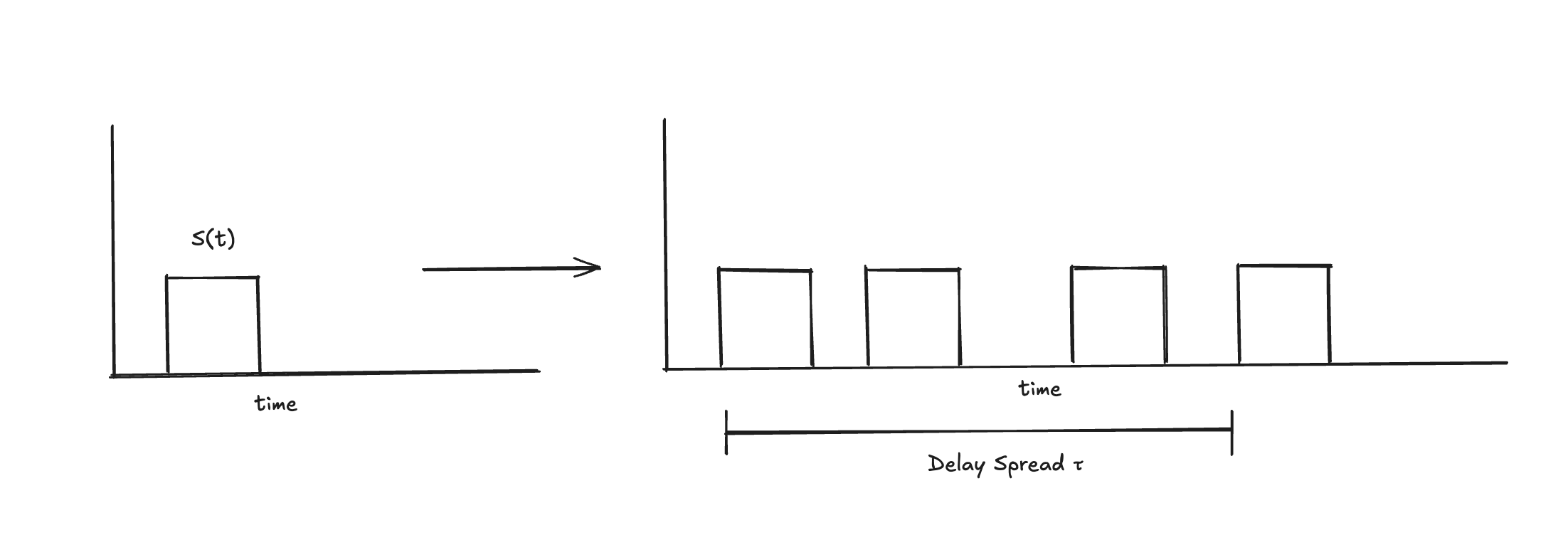
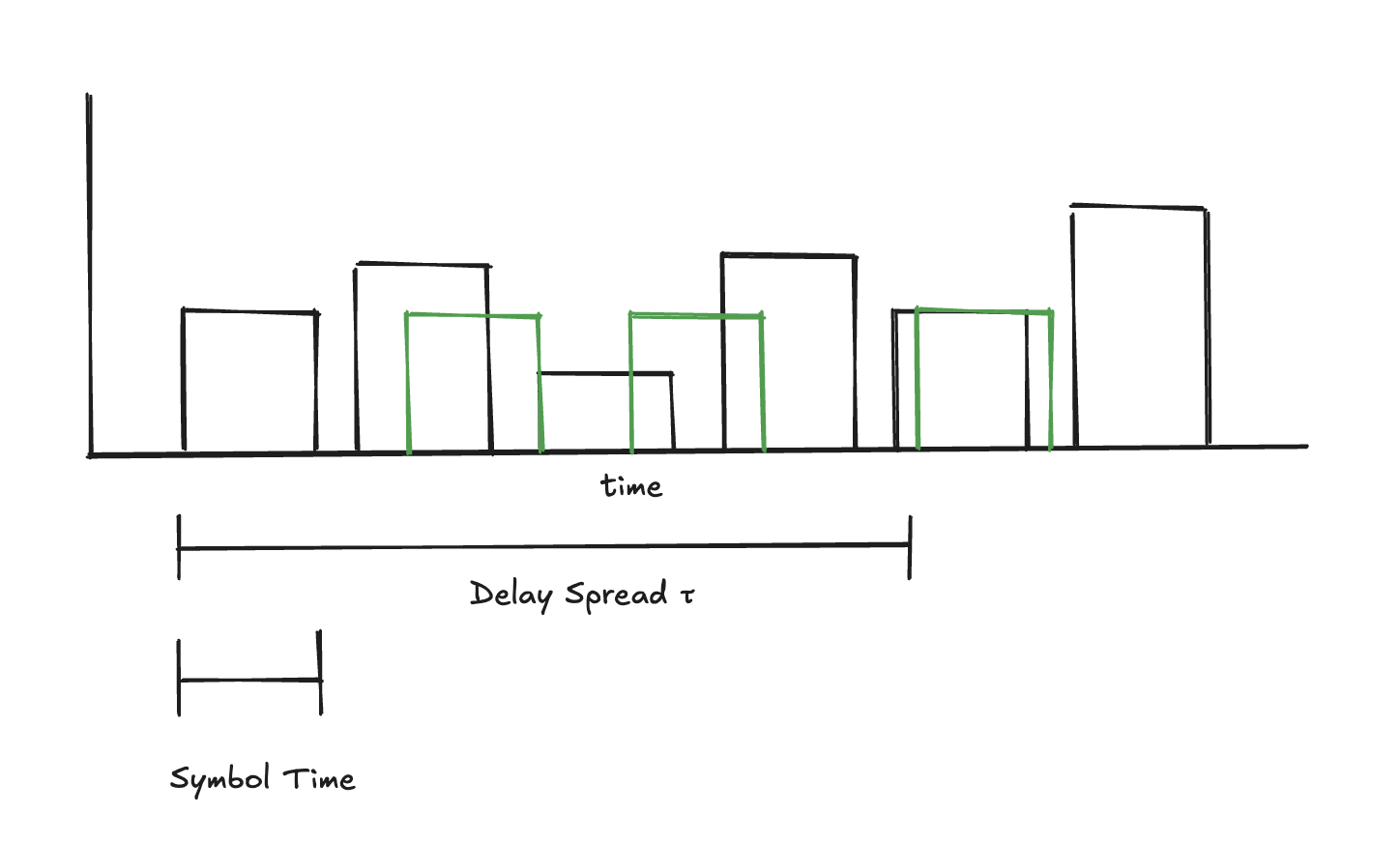
Notice that this is kinda bad. If I send a signal symbol (just imagine it as a quick burst that stores a few bits) and that symbol is shorter than the delay spread, then future symbols will eventually be hit with the “echoes” of the symbols before it. The receiver will get totally confused and won't know how to decipher the data it's getting. This is called Inter-Symbol Interference (ISI). In the diagram below you can see that the black pulses are the symbols we are actually trying to send but it interferes with the green "echoes" of the original symbol since the channel causes the symbol to arrive at different times.

The Frequency Perspective (Coherence Bandwidth)

For simplicity, imagine signals as sine waves. These waves can either add together constructively (boosting the power) or destructively (killing the power). Based on the timing of those echoes, the signals can add up to increase or decrease the amplitude at the receiver. This is heavily dependent on the specific frequencies of the signal and the actual channel (the physical environment we are transmitting through).

Basically, the channel has a frequency response, meaning transmitting some frequencies will result in higher power at the receiver, while other frequencies will just get wiped out.

We don't want the channel itself acting like a random filter that affects which frequencies are attenuated or gained. We want to use a chunk of bandwidth where the frequency response is basically flat. That safe portion of frequencies is called the Coherence Bandwidth (B_c).

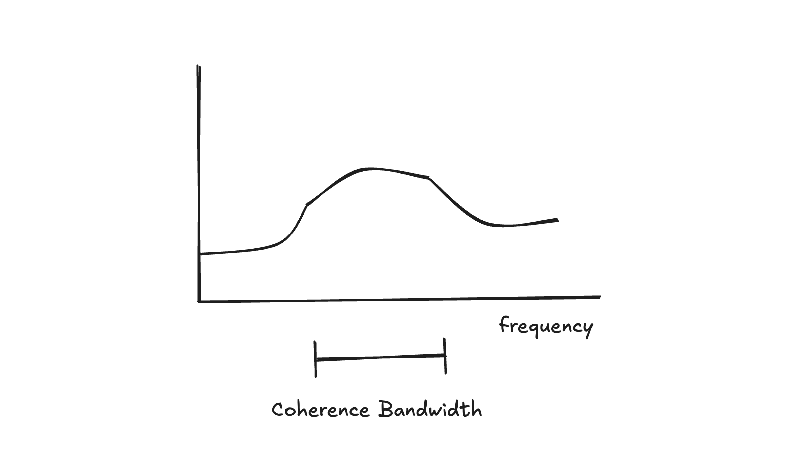
If we are transmitting a signal with a bandwidth that fits inside this coherence bandwidth, we are good, it's called flat fading.

However, if we try to transmit some really wideband signal that's bigger than the coherence bandwidth, that's not good. The channel starts filtering it, causing frequency-selective fading (which leads straight to ISI). Thinking about Shannon's Capacity formula, it basically tells us that the 2 ways we can increase the data rate within a channel, is by either increasing SINR (the amount of signal vs. noise/interference), or just increase the amount of usable bandwidth. We are tackling the latter.

Just think about it like this, the environment dictates the delay spread, and the delay spread dictates the Coherence Bandwidth. If the physical environment has a massive delay spread (lots of late echoes), its Coherence Bandwidth gets squeezed and becomes very narrow. Because of this inverse relationship, B_c \approx \frac{1}{\Delta\tau}. We want our signal's bandwidth to safely fit inside whatever B_c the environment gives us.

The Solution: Multi-Carrier Transmission

So what is the solution? We can use something called multi-carrier transmission, where we divide the massive channel bandwidth (W) into N tiny slots (basically sub-channels).

Each sub-channel gets a tiny slice of bandwidth: \Delta f = \frac{W}{N}.

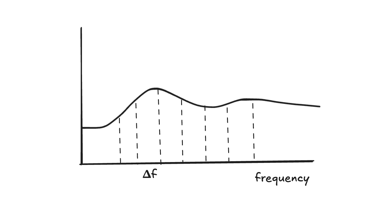
We simply choose N to be large enough so that \frac{W}{N} < B_c.

We take all these sub-channels and send them at the same time!!! Basically, in parallel. We can sendN simultaneous symbols.

Common misconception: This does not necessarily increase the rate at which we send symbols compared to a single carrier. Because we send them in parallel, the time duration of each symbol (T_U) is actually longer. So in the end the rate at which we send symbols is still the same. The thing we are trying to fix right now is using bandwidth larger than the fixed Coherence Bandwidth.

Making the symbol time much longer than the delay spread (T_U \gg \Delta\tau) massively reduces the impact of ISI, but it doesn't kill it completely. The echoes from the previous symbol will still corrupt the very beginning of our current symbol. This is solved with Cyclic Prefix, but I won’t really go into that too much. But think about it, we're increasing symbol time so that ISI is reduced, but we're still keeping the rate that we are sending symbols the same, since we're sending a bunch at the same time! That's basically how we're solving the issue.

The Interference Issue

The important part is: how do we choose \Delta f, the spacing of the frequency blocks after we divide the bandwidth, so that these parallel signals don't interfere with each other? If we don't choose\Delta f carefully, they will become a scrambled mess.

The simple explanation: When we chop a continuous wave into a short burst of time to send a symbol, the energy from that frequency splatters outward and bleeds into neighboring frequencies.

The technical explanation: Remember the Fourier transform! We are transmitting finite blocks of time (the symbol duration, T_U). A rectangular block in the time domain transforms into a Sinc function (\sin(x)/x) in the frequency domain. So when we have neighboring subcarriers, their Sinc functions naturally ripple outward and overlap into each other's frequency lanes. We cannot avoid this overlap in reality.

Basically, yes we are reducing ISI with a longer symbol time and keeping symbol rate the same since we're sending a bunch at once, but this will cause a bunch of interference within each other since we're sending them at the same time, sometimes called Inter-Carrier Interference (ICI). This is where the O in OFDM comes in. We have to choose a frequency spacing so that they DON'T interfere. Divide the frequency band so that they are orthogonal (which is why its called orthogonal frequency division multiplexing). We basically need to choose a \Delta f so that at the exact moment we sample the peak of one signal, all the overlapping ripples from the other frequencies are passing through exactly zero.

THIS IS WHERE ORTHOGONALITY COMES IN!!

If we choose our subcarrier spacing to be exactly \Delta f = \frac{1}{T_U}, we get this mathematical orthogonality. The neighboring subcarriers still overlap heavily, but their Sinc function zero-crossings perfectly align so they don't interfere at the exact sampling points. This specific math trick is what turns standard multi-carrier transmission into specifically OFDM.

Further Optimizations

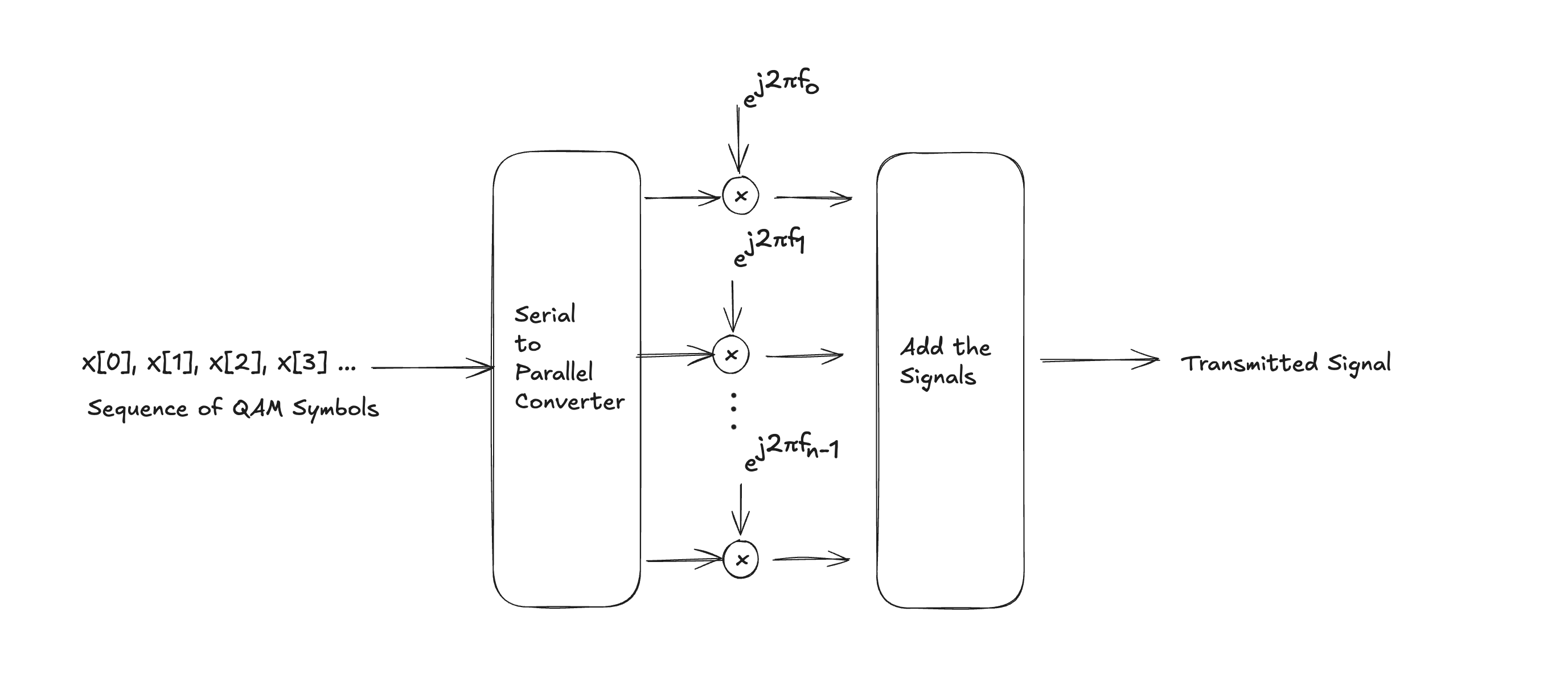
There is another massive way we can optimize this. Notice that if we separate the bandwidth intoN sub-channels, we'd theoretically need N analog mixers and oscillators to multiply the signals by all those different subcarriers. For thousands of subcarriers, that is LOTSSS OF HARDWARE. From a digital design perspective, doing this in analog or instantiating thousands of digital multipliers would be a routing and power nightmare on the silicon.

But notice the math: when we multiply these symbols with the subcarrier frequencies (the complex exponentials) and sum them up, this is literally the exact formula for computing an Inverse Discrete Fourier Transform (IDFT).

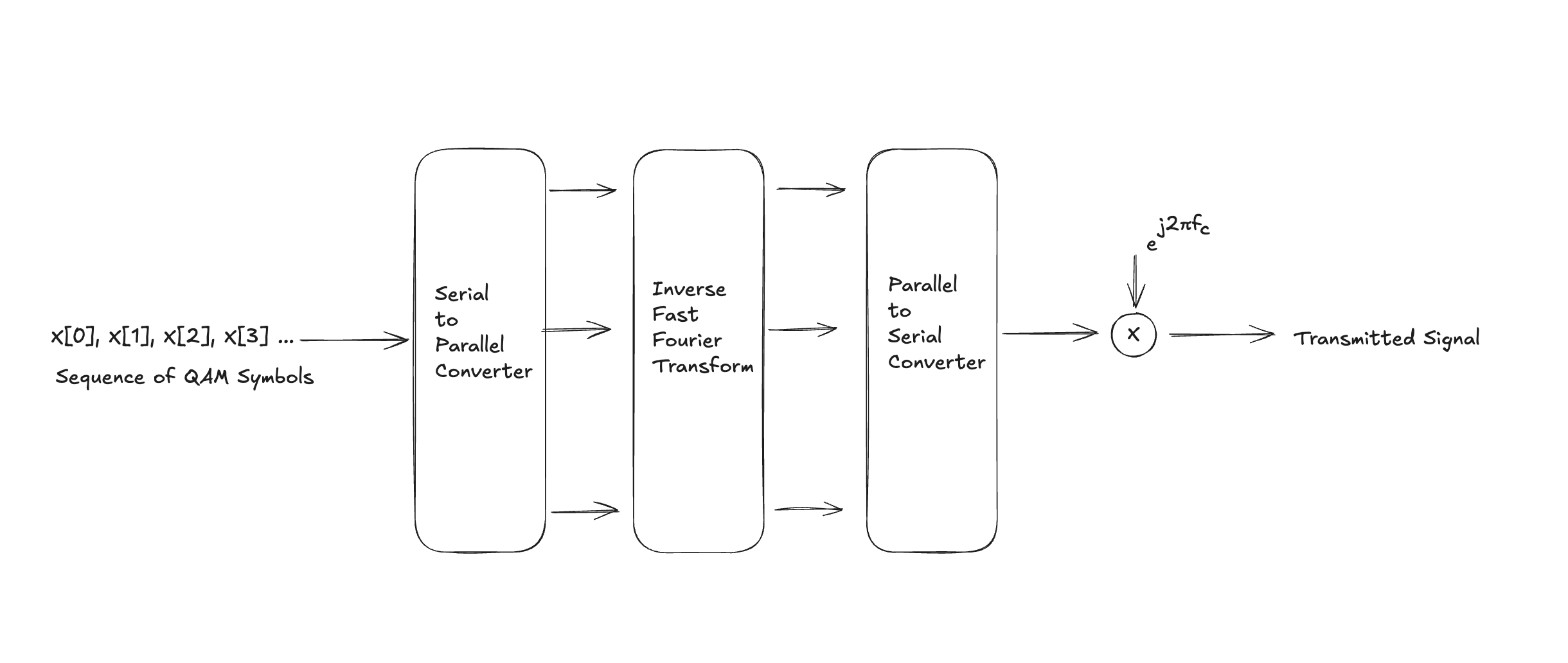
So here is the digital hardware cheat code: all we do in the digital logic is take the intermediate digital symbols (X[0], X[1], X[2], \dots), put them into a serial-to-parallel converter, and then we run them through a highly optimized hardware IFFT block to compute the math perfectly in parallel!

Then we convert that parallel output back to a serial digital stream. We pass that digital stream through a Digital-to-Analog Converter (DAC) to turn those digital numbers into physical analog voltages. Finally, we multiply that analog signal by just 1 single analog mixer to upconvert the whole chunk to the radio frequency, and transmit it.

Simply do the exact reverse (ADC \rightarrow FFT) at the receiver, and you're done! That's basically OFDM.